Background

During one boring afternoon, one of my friend in Boston sent me an interesting plot:

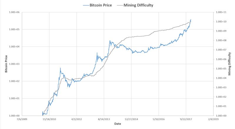
Certainly the correlation between bitcoin price and bitcoin mining difficulty is obvious. But the question imediately pops up in my mind: Why? What is the cause behind this strong correlation?

Let’s start with this simple question: What are those people who devoted into bitcoin mining from the earliest days like?

The answer is simple: they believe in bitcoin and want to drive up the bitocin price.

Based on this simple thought, I come up with a simple model, which models the interaction between bitocoin price, bitcoin mining difficulty, total bitcoin numbers and total bitcoin mining power.

Model

I have to admit that this is a little bit math heavy for some of the users so if you are bored by the math, please just jump the modeling part. For the math expert people, I have to admit that I haven’t done rigorous proofs and everything is questionable here.

I have used stochastic optimal control to model the evolution of bitcoin price and the actions taken by the main bitcoin miners. And eventually use this to show this will leads to the correlation between the mining difficulty and bitcoin price over the past five years which we have discovered in the history data.

The basic assumption of this model is as follows:

The state space we are interested in is in $R^4$ .
$Z(t) = (P(t),D(t),N(t),C(t))$
where $P(t)$ is the ‘bitcoin price’ at time t, $D(t)$ is the ‘mining difficulty’ at time t, $N(t)$ is the ‘total number of coins already been mined’, and $C(t)$ is the current ‘total mining power’ measured in unit TH.
For simplicity we only consider only one main bitcoin miner and that big player can make two kinds of constrained decision at each time: whether to invest more money on mining or to decrease the current mining power. So abstractly the dynamic of the state can be descrbed as:
$\frac{d}{dt}Z(t) = F(Z(t),\nu(t)) , t>0,$ $Z(0) = (P_0,D_0,N_0,C_0)$
where $\nu(t)$ is the control term. $P_0$ is the initial bitcoin price, $D_0$ is the initial bitcoin mining difficulty, etc…

As we mentioned earlier the ‘Big Player’ wants to maximize his profit in long term because he believes in Bitcoin and also wants to minimize his total cost spent on mining. We use the value functional J to represent his earning.
The value functional J is the functional which we want to maximize. Our main assumption here is that the big miner will always hold the mined bitcoin and eventually want to maximize their value with limited control. To write out:
$\nu(t) = sup_{\nu\in A} N(T)\cdot P(t)-\int_{0}^{T} \nu(t) dt$
where A is the admissible control set.

Under this abstract settings, we need to develop a reasonable function F which will somehow recover the dynamic of the whole system.

$\frac{d}{dt}P(t) = P(t)(\mu dt+\sigma_1 dW)-f_{1}(\nu(t))dt$

where $f_{1}$ is a stricty increasing positive function, since adding more mining power will increase the provide of bitcoins and will drive down the price in short time.

$\frac{d}{dt}D(t) = f_{2}(N(t),C(t))dt+\sigma_2 dW$

This has the meaning of the mining difficulty is adjusted by the current mining power and number of coins that has been already mined.

$\frac{d}{dt}N(t) = C_1 C(t)/D(t) dt+\sigma_3 dW$

Means: the number of the coins that already have been minded increases with the speed of current mining power divided by the current mining difficulty.

$\frac{d}{dt}C(t) = (1-C_2)dt+\nu(t)$

This means that the mining rig is going to be out of date with the ratio of $C_2$ and here is the control takes part, we can either increase the mining power which will drag down the price in short term and increase the difficulty or to decrease the mining power to have the opposite effect and hope to have a better payoff in long term.

We can rewrite our model into a more concise and abstract form:

$\frac{d}{dt}\begin{pmatrix}P(t)\\D(t)\\N(t)\\C(t)\end{pmatrix} = \mu(t,P(t),D(t),N(t),C(t),\nu(t))dt+\sigma dW$

where $\mu(t,P(t),D(t),N(t),C(t),\nu(t))= \begin{pmatrix} \mu_1 P(t)-f_{1}(\nu(t))\\f_{2}(N(t),C(t)) \\C_{1}C(t)/D(t)\\ 1-C_{2}+\nu(t)\end{pmatrix}$

dW is a vector of independent white noises.

and $\sigma = \begin{pmatrix}\sigma_{1}\\\sigma_{2} \\\sigma_{3} \\0 \end{pmatrix}$ is the volatilitly constant.

In order to apply the Dynamic Programming Principle(DPP), we have to check that our model meets the 4 assumptions:

Assumption 1: to be added…

Assumption 2: The affect of the control $\nu$ is causal, as we can see any two same control will give us the same result in the sense of expectation.

Assumption 3: Concatenating two admissible controls will also give us an admissible control by the construction of our admissible controls set.

Assumption 4: It is easy and obvious to see that our value function J is additive. Now we are in good shape to apply the Ito’s formula to derive the Dynamic Programming Equation(DPE). In our finite horizon setting, the DPE equation reads:

$-\frac{\partial}{\partial t} v(t,P,D,N,C)+H(P,D,N,C,t,\nabla v(t,P,D,N,C),D^{2}v(t,P,D,N,C)) = 0$

where

$H()$ plug in our stochastic dynamic system and choosing simple form of functions $f_{1},f_{2}$,we have:

Simulation

I have runned 1000 Monte Carlo Simulations, the code are provided below:

import numpy as np
import math
import matplotlib.pyplot as plt
from scipy.stats import norm

# simply forward the stochastic ODE using explicit scheme
NN = 500
P = [0]* NN
D = [0]* NN
N = [0]* NN
C = [0]* NN
mu= [0]* NN
dt = 0.01
mu_1 = 1
sigma_1 = 0.1
C1 = 5
C2 = 0.99

# initial conditon
P[0] = 100
D[0] = 100
N[0] = 100
C[0] = 100

def f1(x):
    return x*x*x

def f1primeinverse(x):
    return 1

def f2(x,y):
    return x*y

for j in range(1,100):
    for i in range(1,NN):
        #mu_i = np.exp(np.random.normal(0,1))
        mu_i = np.sqrt((C[i-1]*P[i-1]/(D[i-1]*D[i-1]))+(1/N[i-1]))
        dP = (mu_1*P[i-1]-f1(mu_i))*dt+ P[i-1]*sigma_1*np.random.normal(0,1)
        dD = f2(N[i-1],C[i-1])*dt
        dN = (C1*C[i-1]/D[i-1])*dt # dN should be a constant according to the bitcoin settings
        dC = C[i-1]*(1-C2+mu_i)*dt
        #print dP,dD,dN,dC
        P[i] = P[i-1]+dP
        D[i] = D[i-1]+dD
        N[i] = N[i-1]+dN
        C[i] = C[i-1]+dC
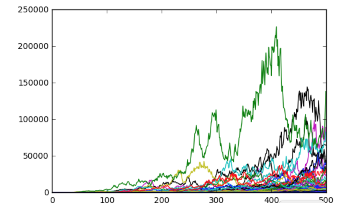
    plt.plot(P)
plt.show()

Result

BTC Price

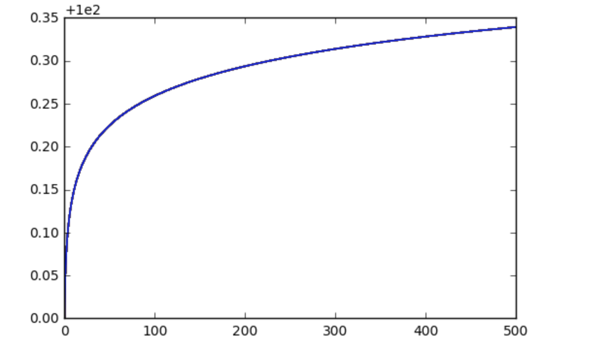
Total number of bitcoins

BTC Mining Difficulty

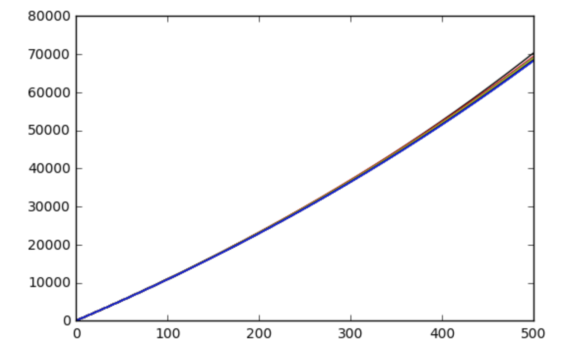The result has showed the time evolution of the probabilty density of the Bitcoin Price, Mining Difficulty, Total Number of Coins.

We can see that this model has an upper bound of total number of coins which meets well with the design of Bitcoin.

And the Price has certain correlation with mining difficulty and both tends to grow exponentially.

BitCoin TipJar

BTC Address: 112ca6RbrargroNBvosVZgY7BzmTsm7hhT

Ethereum TipJar

ETH Address: 0x40B693679D7984aEb0062C25Ca3d406ECD2Aff41