AR-Retrofit and ReSkip: Attention Residuals on a Frozen Backbone

Part 3 of a series on attention residuals and AR-Retrofit. Part 1 set up the residual stream; Part 2 replaced the fixed + with learned attention over depth.

The problem this post is about

Attention Residuals are nice. They give us input-dependent depth combination and a pre-execution routing signal. But the recipe in Part 2 assumes you are training from scratch.

The models we actually want to deploy — Qwen3, Llama, the VLM backbones built on top of them — were trained with the fixed scalar-1 +. Their weights are co-adapted to that recipe: block \(l\) expects its input to be exactly \(x_{l-1}\), the sum of everything written into the stream up through block \(l-1\). Swap the + for a softmax over \(\{h_0, \ldots, h_{l-1}\}\) and the block sees an input from a distribution it has never been trained on. Performance collapses.

A full retrain is the obvious answer and the one we cannot afford. So the question is:

Can we keep the pretrained backbone frozen, add attention residuals as a side-channel, and recover the benefits of AttnRes for under half a percent of new parameters?

The answer is yes, and the design that makes it work is AR-Retrofit. The inference-time payoff — using the learned routing weights to skip blocks — is ReSkip. This post is the recipe and the things that almost worked but did not.

What we need to preserve

Two things are non-negotiable when retrofitting onto a frozen backbone:

1. Identity at initialization. At training step zero, the modified model must produce exactly the same outputs as the pretrained model, up to numerical noise. Otherwise we start training from a worse-than-pretrained point and may never catch up.
2. Input manifold preservation. Each frozen block \(\mathrm{Block}_n\) was trained to expect inputs from a specific distribution. The retrofit must not push that distribution too far. Direct replacement of \(x_n\) with a softmax-weighted \(r_n = \sum_i \alpha_{i \to n} h_i\) does push it too far — even when \(\alpha\) is initialized to peak on \(n-1\), the soft mass on other \(i\) shifts the input enough that frozen blocks degrade.

Both constraints point in the same direction: the retrofit cannot be a replacement of the residual, it has to be a correction on top of it, gated to start at zero and ramp up.

The AR-Retrofit recipe

Here is the full recipe between two frozen blocks. Let \(h_{n-1}\) be the output of the previous block (what the standard residual stream would have carried into block \(n\)).

\[\begin{aligned} \tilde k_i &= \mathrm{RMSNorm}(h_i) + b_i \\ \alpha_{i \to n} &= \mathrm{softmax}_i\!\left(\frac{w_n^\top \tilde k_i}{\sqrt d}\right), \quad i = 0, \ldots, n-1 \\ r_n &= \sum_{i=0}^{n-1} \alpha_{i \to n}\, h_i \\ x_n &= h_{n-1} \;+\; \gamma_n \cdot A_n\!\left(r_n - h_{n-1}\right) \\ h_n &= \mathrm{Block}_n(x_n) \quad (\text{frozen}) \end{aligned}\]

with the bottleneck adapter \(A_n(u) = W_{\text{up}}\, \sigma(W_{\text{down}}\, u)\) at rank \(r = 256\), and gate \(\gamma_n\) a learnable scalar following a curriculum from \(0\) at the start of training to \(1\) at roughly 30% of the way through.

Five design choices are doing real work here. Each was the wrong answer at least once on the way to this one.

1. The base path is still the standard residual

Notice that the first term of \(x_n\) is just \(h_{n-1}\). If you delete the entire AR-Retrofit machinery you get back the original model exactly. The retrofit only ever adds a correction; it never replaces the base.

This is what “identity at initialization” buys you. At \(\gamma_n = 0\) the correction term vanishes, \(x_n = h_{n-1}\), and the model is the frozen backbone running unchanged. We can verify this empirically — at \(\gamma = 0\) the retrofit reproduces base model outputs to bf16 noise.

2. The correction is on \((r_n - h_{n-1})\), not \(r_n\)

The thing fed into the adapter is the difference between the routed state and the standard residual. If \(\alpha\) collapses to one-hot at \(i = n-1\), then \(r_n = h_{n-1}\), the difference is zero, and the adapter has nothing to do. We have not perturbed the input manifold at all.

This is what lets the router learn freely. A router that is forced to do something useful even when the standard residual is fine ends up corrupting easy cases. By subtracting off the standard residual we make the correction optional — the router only matters when the routed combination genuinely differs from the previous-state baseline.

3. \(\gamma\) curriculum, \(0 \to 1\) over the first 30%

A learnable gate alone is not enough. If \(\gamma\) is initialized small but free, gradient signal pushes it up before the router and adapter have learned anything coherent — and a half-trained router driving a half-trained adapter at non-trivial \(\gamma\) pushes the frozen block off its input manifold.

The fix is to schedule \(\gamma\) explicitly. Start at exactly zero. Hold for a few percent of training so the router and adapter can train on a clean gradient signal (gradients still flow even at \(\gamma = 0\) because the adapter’s up-projection is initialized nonzero). Then ramp linearly to one over the next 25–30% of training. By the time the gate is fully open, the modules have learned a correction worth applying.

4. The adapter is low rank

At rank \(r \approx 256\) on \(d\) in the low thousands, the adapter dominates the new-parameter cost — but the cost is small. The whole side-channel ends up well under half a percent of a multi-billion-parameter backbone.

There is no obvious reason higher rank would help. The router does the interesting work — choosing which prior states to combine. The adapter only has to express a small correction in the direction the router chose; a low-rank bottleneck is plenty.

5. Block-level granularity

Do not apply AR-Retrofit per layer. Group \(L \approx 4\) contiguous transformer layers into a block and apply one retrofit per block. This matches Kimi’s from-scratch finding for AttnRes (\(S \in \{2, 4, 8\}\) all work reasonably; finer than that and the router has nothing useful to say between adjacent layers).

Block granularity also keeps the router’s pre-execution signal interpretable: “block \(n\) matters” is a useful unit. “Layer 37 matters” rarely is.

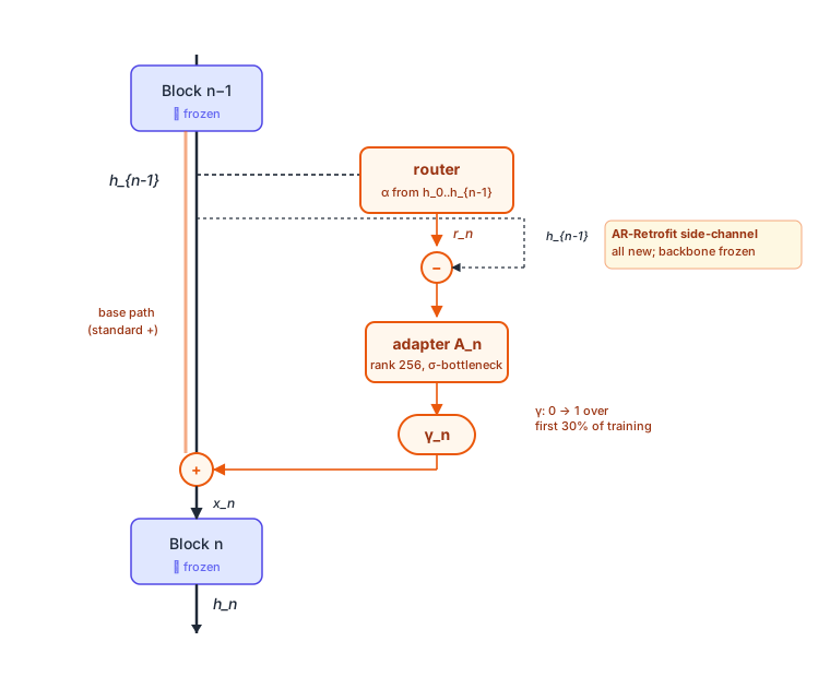
Diagram 5. The AR-Retrofit side-channel sitting between two frozen blocks. The base path (amber spine) is the standard residual, still present. Off to the side, the router forms \(r_n\), the difference \(r_n - h_{n-1}\) is run through a low-rank adapter, multiplied by the scalar gate \(\gamma_n\), and added back to the stream. At \(\gamma_n = 0\) the side-channel is silent and the model reproduces the frozen backbone exactly.

Training the retrofit

The frozen backbone is the teacher. The retrofit is trained with a three-term loss:

\[\mathcal{L} = \underbrace{\mathrm{CE}(x, y)}_{\text{full path}} \;+\; \lambda_{\text{kl}}\, \underbrace{\mathrm{KL}\!\big(p_{\text{teacher}} \,\|\, p_{\text{skip}}\big)}_{\text{makes blocks skip-friendly}} \;-\; \lambda_{\text{ent}}\, \underbrace{\mathbb{E}\big[H(\alpha)\big]}_{\text{prevents collapse}}\]

• Full-path CE. Ordinary next-token prediction, end-to-end through the retrofitted model with all blocks active.
• Skip-branch KL. On each step, randomly mask one block (replace \(\mathrm{Block}_n\) with the identity for the rest of the forward) and distill from the unmodified frozen teacher. This is the term that makes blocks individually skippable later. Without it, \(\alpha\) learns a routing the model happens to like but cannot survive any block being absent.
• Entropy bonus. A small reward on \(\mathbb{E}[H(\alpha)]\) keeps the softmax from prematurely collapsing onto a single source. Without it, \(\alpha\) converges to near one-hot at \(i = n-1\) — which trains fine but throws away the entire point of the mechanism.

The teacher is the unmodified frozen backbone; no separate teacher model is needed.

Why not the simpler thing?

Three nearby designs do not work, and the reasons are instructive.

Observer-only routing. Compute \(\alpha\) but do not let it affect the forward pass — just use it as a diagnostic. This gives you the routing signal “for free” but the routing weights end up uncorrelated with anything useful, because nothing in the loss makes them correspond to block importance. You cannot get a useful signal out of a module the rest of the network is ignoring.

Direct interpolation toward \(r_n\). Set \(x_n = (1 - \gamma) h_{n-1} + \gamma\, r_n\) instead of using a low-rank adapter on the difference. Frozen blocks degrade quickly as \(\gamma\) rises, because the soft mass over earlier \(h_i\) pushes block \(n\)’s input off the distribution it was pretrained on. The adapter on \((r_n - h_{n-1})\) exists exactly to express a small correction; direct interpolation can express arbitrarily large ones, and the gradient signal pushes it that way.

\(\gamma\)-free, always-on adapter. Replace \(\gamma_n \cdot A_n(r_n - h_{n-1})\) with just \(A_n(r_n - h_{n-1})\) — initialize \(A_n\) near zero and trust SGD. This loses the identity-at-init guarantee. Even with conservative init, the first many thousand steps inject non-trivial noise into frozen-block inputs, denting perplexity in ways the model struggles to recover from. The explicit curriculum on \(\gamma\) is what makes the bridge from “exactly the base model” to “fully retrofitted” smooth.

The pattern across the three: the routing module needs to do something for its weights to mean something, but what it does must be a correction small enough that the frozen backbone tolerates it. The recipe — gated, low-rank, on the difference — is the smallest configuration that satisfies both.

ReSkip: using \(\alpha\) at inference

Now we have a model where \(\alpha_{i \to n}\) is a real, trained, pre-execution signal about how block \(n\) is using its predecessors. Two diagnostics make it usable as a skip signal.

Routing importance of block \(n\):

\[I(n) = \max_{l > n} \mathbb{E}\!\left[\alpha_{n \to l}\right]\]

This is the largest expected attention any future block places on \(h_n\). If \(I(n)\) is small, no downstream block cares much about \(h_n\) on average.

Ablation cost of block \(n\):

\[A(n) = \frac{\mathrm{PPL}(\text{block } n \text{ removed})}{\mathrm{PPL}(\text{full})}\]

A direct measurement: how much worse does the model get if we just drop block \(n\)? Computed once on a calibration set.

Neither alone is enough. \(I(n)\) low does not guarantee block \(n\) is safe to drop — a low-routing block can still be doing load-bearing work that happens to flow through the standard residual path. \(A(n)\) low does guarantee safety, but it is a property of the calibration set; it does not tell us when a particular input is a good time to skip.

So we use them together. Offline, we compute \(A(n)\) for every \(n\) and form the eligible set \(P = \{n : A(n) < 1 + \delta\}\) — blocks that ablation tells us are safe to drop. Online, for each input, we look at the recent routing weight onto \(h_{n-1}\):

\[w_{\text{recent}}(n) = \mathbb{E}_{\text{recent tokens}}\!\left[\alpha_{n-1 \to n}\right]\]

and skip block \(n\) when

\[w_{\text{recent}}(n) > \tau_n \quad\text{AND}\quad n \in P \quad\text{AND}\quad |\text{skipped so far}| < M_{\max}\]

where \(\tau_n\) is a calibrated quantile threshold per block, and \(M_{\max}\) caps how many blocks we are willing to drop. The first condition is the per-input decision; the second is the offline safety net; the third is a guardrail against pathological inputs that would tempt the policy into skipping everything.

The condition \(w_{\text{recent}}(n) > \tau_n\) is intentionally counterintuitive. A high routing weight onto the previous-state means block \(n\)’s input was mostly the standard residual — the routing module is not pulling new information from earlier states. That is exactly when block \(n\)’s contribution is most likely to be a small refinement that we can afford to skip.

A margin-preservation argument

A simple property explains why this works empirically. Let \(\Delta(x)\) be the top-1 minus top-2 score at the output under the full model, and \(\varepsilon(x)\) the maximum logit perturbation introduced by skipping eligible blocks. Then

\[2\varepsilon(x) < \Delta(x) \;\Longrightarrow\; \text{top-1 prediction unchanged.}\]

In other words: as long as the perturbation introduced by skipping is smaller than half the margin, the prediction is identical. The eligible set \(P\) and the threshold \(\tau_n\) are calibrated to keep \(\varepsilon\) small; the entropy-regularized routing keeps \(\Delta\) healthy. The two together explain why ReSkip can drop multiple blocks per forward without measurable accuracy loss on most inputs.

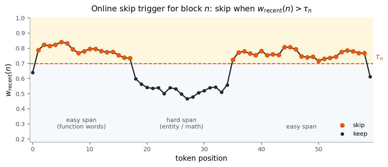
Diagram 6. Online skip trigger for a single block over a sequence (synthetic, illustrative). The dashed line is the calibrated threshold \(\tau_n\). Tokens above the line trigger a skip (amber); tokens below are kept (dark). Easy spans — function words, common continuations — cluster above the threshold; hard spans — entity-heavy clauses, math — cluster below.

What you should expect to see

If the recipe is doing its job, three things should hold up empirically:

• Step-zero parity. At \(\gamma = 0\) the retrofitted model is the frozen backbone, output-for-output (up to numerical precision). This is a verifiable invariant, not an aspiration — if you do not see it, the adapter or normalization is wrong.
• Modest gains over the base model. The routing module gets to redistribute mass over depth, which on most benchmarks buys a small but consistent improvement over the frozen model. Magnitudes will depend on the family, the scale, and the SFT mix — but small-positive is the regime to look for. Large gains on a single benchmark are usually a sign of overfit calibration, not a sign of an unusually good recipe.
• Skippable budget under ReSkip. A trained \(\alpha\) should give you several blocks-per-forward of skip budget at near-base accuracy. If ReSkip is not free or near-free in expectation, either the eligible set \(P\) is too generous or the entropy regularization was too weak and \(\alpha\) collapsed.

Parameter cost is the easy part: at adapter rank 256, the side-channel is well under half a percent of a multi-billion-parameter backbone. The router and bottleneck adapter are tiny compared to the FFN they sit next to.

Things to watch for

A few failure modes that this design does not automatically protect against. Worth knowing in advance.

Family transfer is not free. The recipe was developed against a particular pretrained family. The reasoning behind each choice (identity-at-init via \(\gamma\) curriculum, low-rank correction on the difference, etc.) is general, but the empirical claim that block-level granularity at \(L = 4\) is the right plateau leans on the specific block structure of the backbone. Different attention/FFN aspect ratios may want different groupings.

SFT mix is load-bearing. A router that is supposed to learn to route gets a much weaker training signal from a narrow SFT mix. Mixes that are too narrow or too task-specific tend to push \(\alpha\) toward near-one-hot routing — the loss is fine, but the routing signal becomes vestigial and you have effectively rebuilt the standard residual at three times the cost. Diversity in the SFT data is what keeps the router alive.

Block-level, not per-token, routing. The router decides per-block, not per-token. This bounds how fine-grained the adaptive computation can be and is qualitatively different from MoD-style per-token approaches. Whether that matters depends on your workload; for tasks dominated by uniform-difficulty tokens it does not, for heavily mixed-difficulty workloads it can.

ReSkip thresholds are deployment-specific. Calibrating \(\tau_n\) and the eligible set \(P\) on text and then deploying onto, say, a VLA action stream is the kind of thing that looks like it should work and does not. Per-modality recalibration is a real cost; expect to budget for it.

Wall-clock is not the same as parameter cost. The router and adapter introduce small sequential dependencies between the routing computation and the block forward. On accelerators with aggressive kernel fusion, this can eat into the theoretical inference savings from ReSkip. Measure on your target hardware, not just on the box where you trained.

Closing the loop

We started Part 1 wondering what was hiding in the residual +. The answer, three posts later, is: a fixed-weight, input-independent identity that can be replaced with a learned, input-dependent softmax which gives us a usable pre-execution routing signal. That signal is useful for adaptive computation, useful for interpretability (the per-block \(w_l\) is a real artifact you can read), and useful for inference-time block skipping that pays back the cost of the routing module itself.

The retrofit story is the practical version of that idea: you do not need to retrain a 4B-parameter backbone to get most of the benefit. Under half a percent new parameters, a gated low-rank correction on the difference from the standard residual, and a curriculum that bridges identity-at-init to a fully active router. Plus a skip policy that uses the routing weights to recover the cost.

The most interesting open question is whether the routing weights are interpretable in a stronger sense — whether \(w_l\) across a trained model encodes anything like a learned computational graph over depth. That is a longer story than this series. For now: the + is a stand-in, and there are useful things to put in its place.