Attention, the Residual Stream, and What's Hiding in the "+"

Part 1 of a series on attention residuals and AR-Retrofit.

Why this series

The Annotated Transformer derives attention beautifully. But it treats x + Sublayer(LayerNorm(x)) as a given — a single line of code. That + is doing more work than it looks, and it is also the place where a recent line of research opens up interesting possibilities.

This series builds up to an idea — call it AR-Retrofit — for converting a pretrained decoder into an adaptive-depth model without retraining the backbone. To explain it cleanly we need three pieces:

1. (this post) Attention, compactly, and what the residual is actually doing.
2. (next) Attention Residuals: making the depth combination learned and input-dependent.
3. (after that) AR-Retrofit and ReSkip: retrofitting attention residuals into a frozen pretrained model, and using the resulting routing signal to skip blocks at inference time.

We are not going to re-derive attention from scratch — the Annotated Transformer already does that, and you should read it first if you have not. We will move quickly through the parts that matter for the rest of the series, and slow down on the residual.

Attention in one page

Given a sequence of tokens with hidden states \(X \in \mathbb{R}^{n \times d}\), attention produces a new sequence by letting each position pull information from the others. The mechanism is three steps:

1. Project each row to a query, key, and value:

1. Compute attention weights as scaled dot-products between queries and keys, normalized with softmax:

1. Take a weighted average of values:

The \(\sqrt{d_k}\) keeps the dot-product variance from blowing up at large \(d_k\), where the softmax would otherwise collapse onto a single key.

Multi-head attention runs \(h\) copies of this in parallel on different projections, concatenates them, and applies an output projection:

def attention(Q, K, V):
    scores  = Q @ K.T / sqrt(d_k)
    weights = softmax(scores, dim=-1)
    return weights @ V

def multihead(X):
    heads = [attention(X @ Wq[i], X @ Wk[i], X @ Wv[i]) for i in range(h)]
    return concat(heads) @ Wo

That is the across-tokens mixing operation. In a decoder the score matrix \(A\) is masked so position \(t\) can only attend to positions \(\le t\).

The transformer block

A transformer block alternates between attention (token mixing) and a feed-forward network (channel mixing):

with \(\mathrm{FFN}(u) = W_2\,\sigma(W_1 u)\). This is the pre-norm variant; modern decoders almost universally use pre-norm because it trains more stably at depth.

Two things are happening in each sub-layer:

• LayerNorm rescales the input before the sublayer.
• The residual + adds the sublayer’s output back to its input.

The first is a normalization and we will not say more about it. The second is the focus of this post.

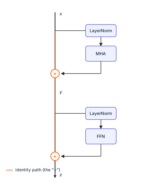
Diagram 1. A single transformer block. The hidden state \(x\) flows top-to-bottom. Two side-cars branch off — first MHA, then FFN — each preceded by LayerNorm and rejoined to the main path with a +. The amber spine is the straight-through identity path that the two + lines preserve.

Three views of the residual

The recipe \(x_l = x_{l-1} + f_l(\mathrm{LN}(x_{l-1}))\) — add the sublayer’s output to its input with weight 1 — is doing three things at once. Any one of them would justify the design; together they are why every modern transformer has a residual stream.

1. Gradient flow

Without residuals, a deep stack compounds Jacobians:

If those Jacobians have spectral norm \(< 1\), the gradient vanishes; if \(> 1\), it explodes. With residuals,

The identity term keeps the gradient from vanishing — there is always a path from the loss back to early layers that does not pass through any nonlinear transformation. This is the original ResNet motivation, and it is what lets transformers stack to dozens or hundreds of blocks without training pathology.

2. Identity at initialization

If \(f_l\) is initialized so that \(\mathbb{E}\!\left[\|f_l(x)\|\right] \ll \|x\|\) — which is what reasonable init schemes give you — then at step zero the block is approximately the identity:

Training is then learning a deviation from identity:

This is iterative refinement at the architectural level. Each block does not transform \(x\) into a fundamentally different thing; it nudges \(x\) in a direction that turns out to be useful for the loss.

3. The residual stream as working memory

This is the view that matters most for the rest of the series. The sequence

is not a sequence of progressively more abstract feature maps. It is a single \(d\)-dimensional buffer that every block reads from and writes to.

Each block:

• reads from \(x_{l-1}\) via LayerNorm and the sublayer’s input projections,
• writes to \(x_l\) by adding its output back,
• and does not overwrite what was already there — earlier content is preserved by the identity path.

This perspective comes from mechanistic-interpretability work (Elhage et al., 2021, A Mathematical Framework for Transformer Circuits), which calls \(x_l\) the residual stream. Different blocks learn to write information into different subspaces of the stream; later blocks learn to read those subspaces. The stream is a shared communication channel, not a pipeline of progressively transformed features.

Once you see it this way, the residual + stops looking like a stability hack and starts looking like the architectural commitment that makes the rest of the system work.

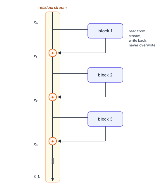
Diagram 2. The residual stream as a single \(d\)-dimensional buffer running top-to-bottom. Blocks 1..L are side-cars: each reads from the stream, computes, and writes its output back with a +. Earlier content is never overwritten.

What is hiding in the “+”

The residual stream view makes one thing very obvious: every block’s output is added to the stream with a fixed weight of 1. Every block, every layer, every input — same scalar. The combination rule is

Why 1? Because that is the identity element. It is the obvious choice when you do not have anything better.

But once we view \(x_l\) as a write into a shared stream, two questions get hard to ignore:

• Why should block \(l\) only see the previous state \(x_{l-1}\)? It could read from \(x_0, x_1, \ldots, x_{l-1}\) — every state is already computed and sitting in memory. The information is right there.
• Why should the combination weights be a fixed scalar 1? Some inputs might benefit from drawing heavily on what block 3 wrote and ignoring block 7; another input might want the opposite.

This is exactly the thing attention was invented for in a different context — letting a query selectively combine multiple sources. So:

What if we used attention not across tokens, but across depth?

That is the move in the next post.

Looking ahead

In Part 2 we will see how Attention Residuals (Kimi Team, 2026) replace the fixed + with a learned attention over previous block outputs. Each block computes a softmax over \(\{x_0, x_1, \ldots, x_{l-1}\}\) and reads a routed combination. This buys two things:

1. The depth combination becomes input-dependent — different inputs traverse different effective paths through the stack.
2. The routing signal is available before the block runs, which turns out to be useful for adaptive computation.

In Part 3 we get to the practical problem: existing pretrained models — Qwen, Llama, the VLM backbones we actually want to deploy — were trained with the fixed +. Can we retrofit attention residuals into them without retraining the backbone? That is the question AR-Retrofit tries to answer, and the design that falls out of taking it seriously is the topic of the last post.